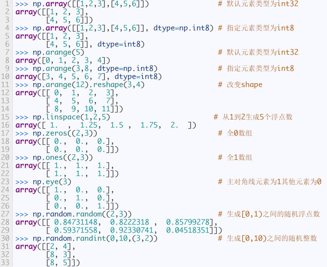
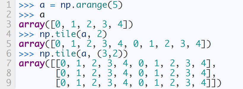
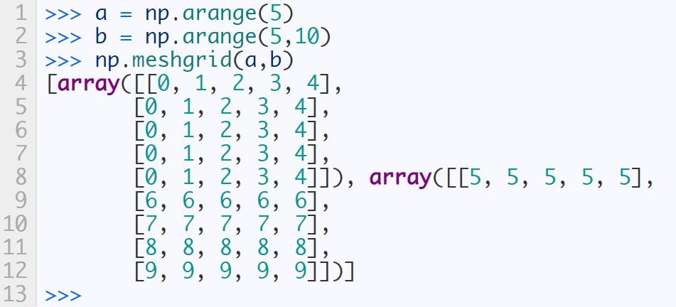
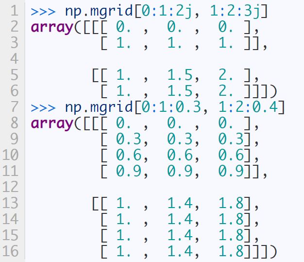
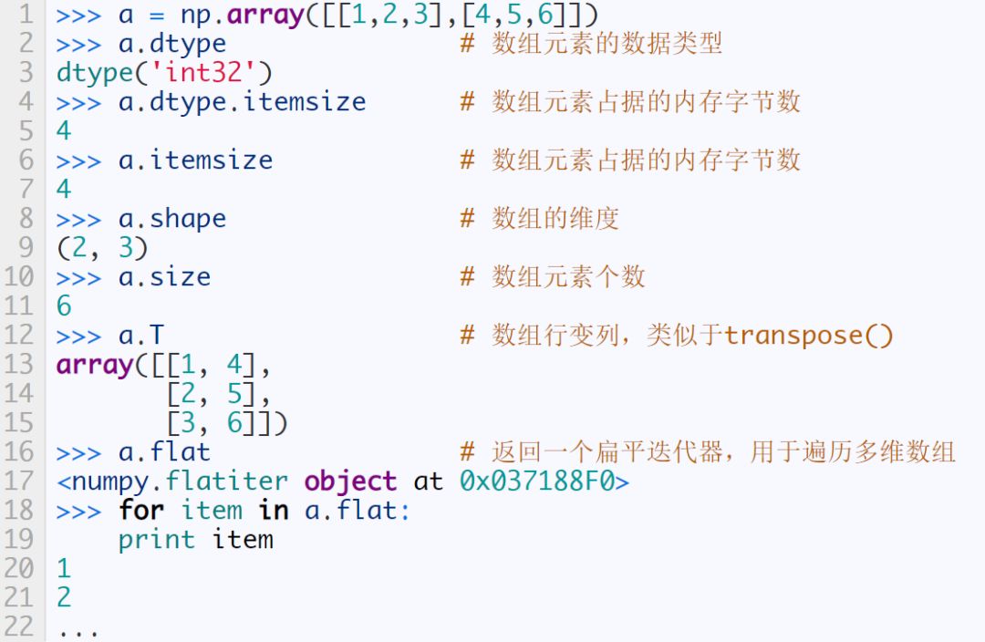
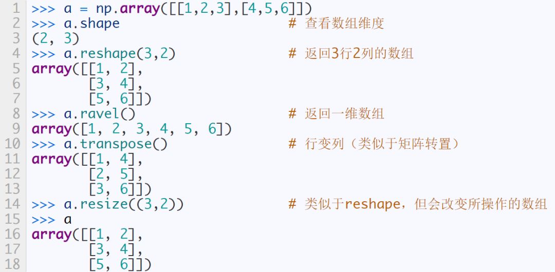
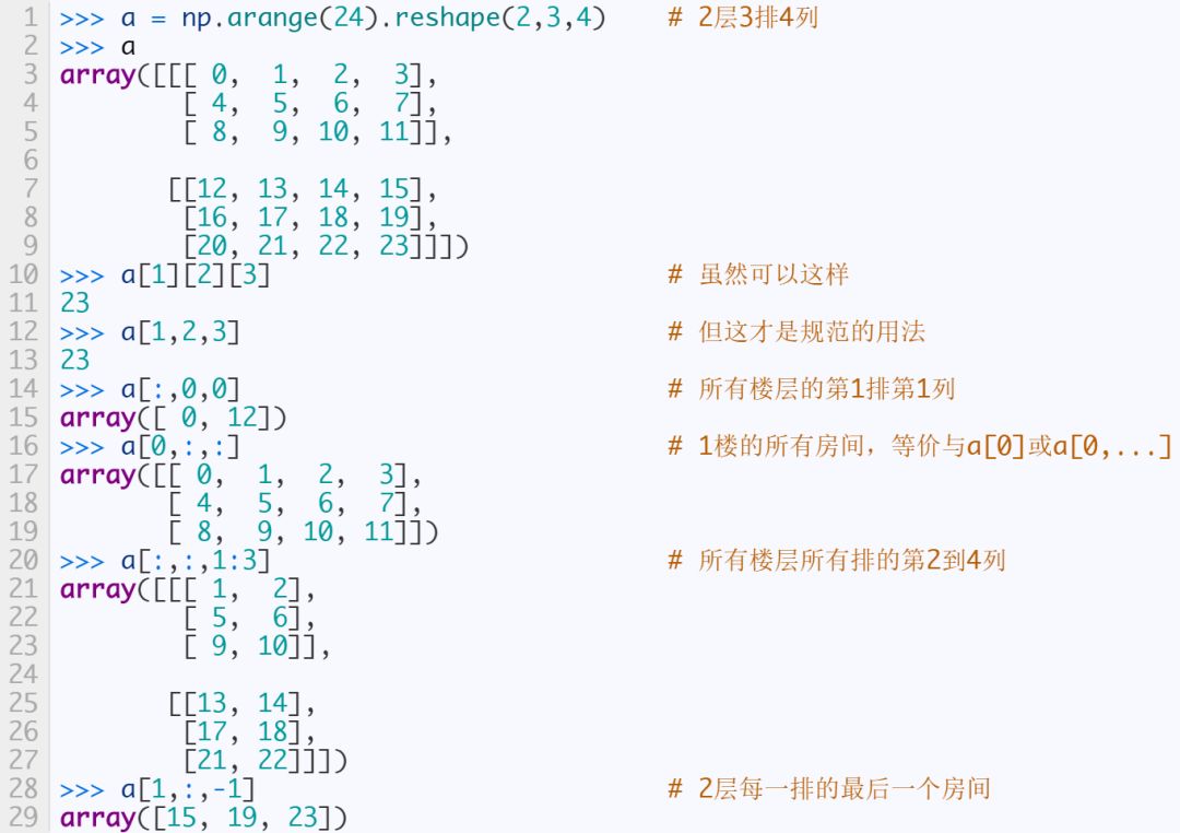
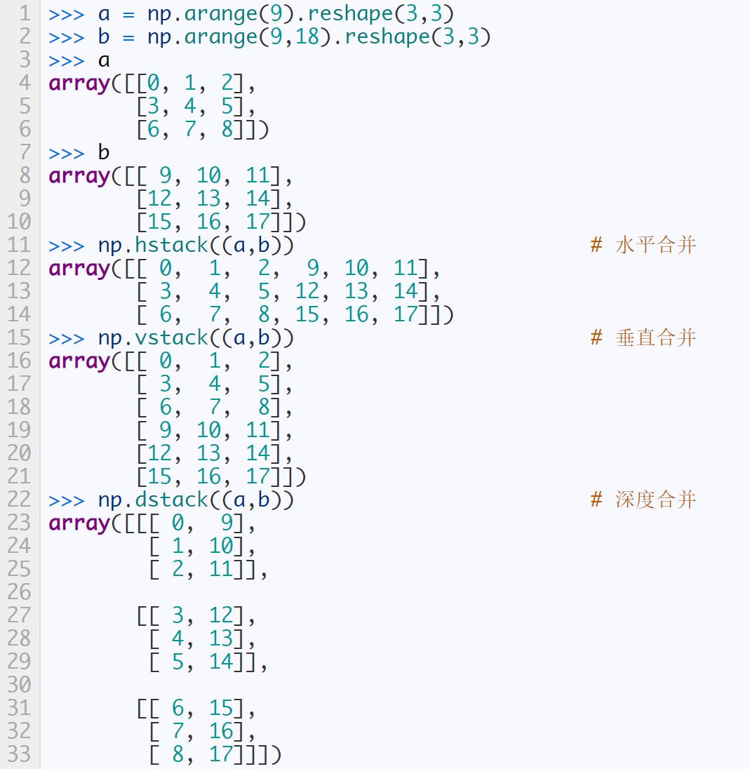
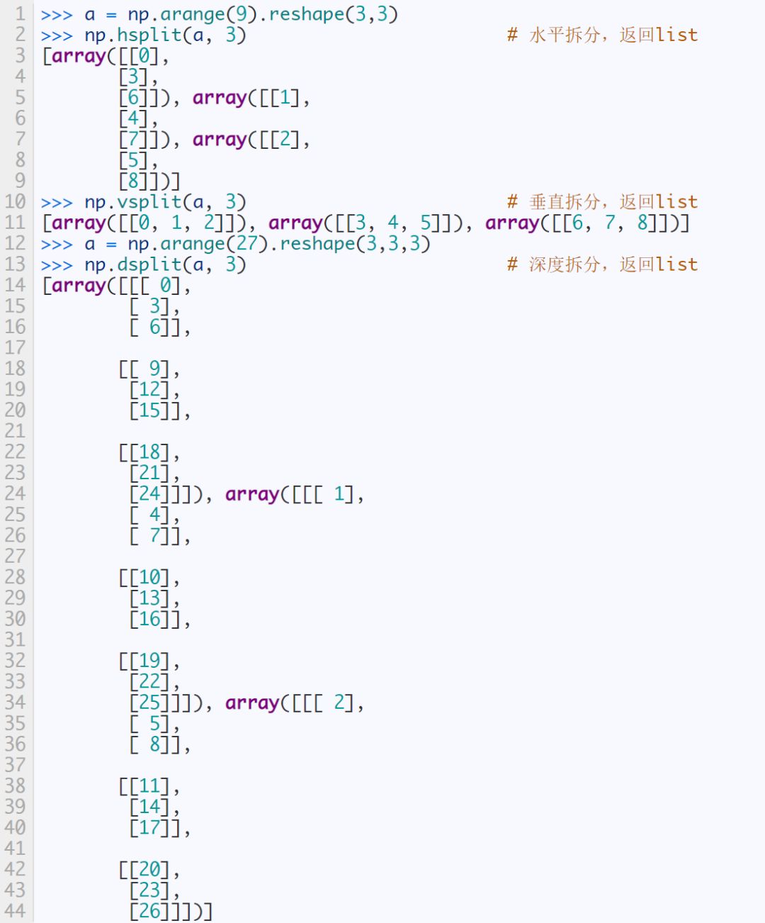
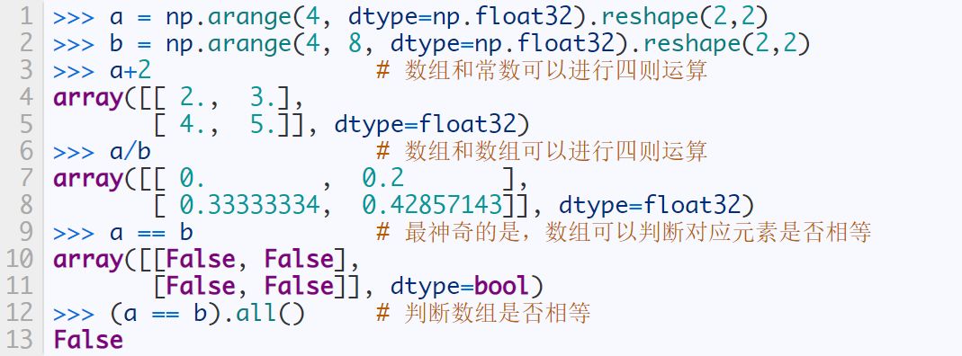
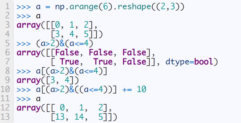
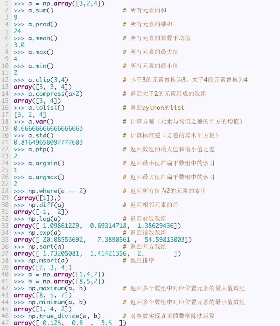
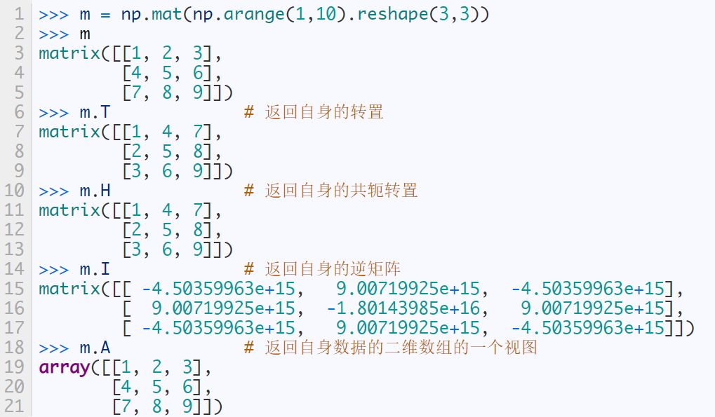
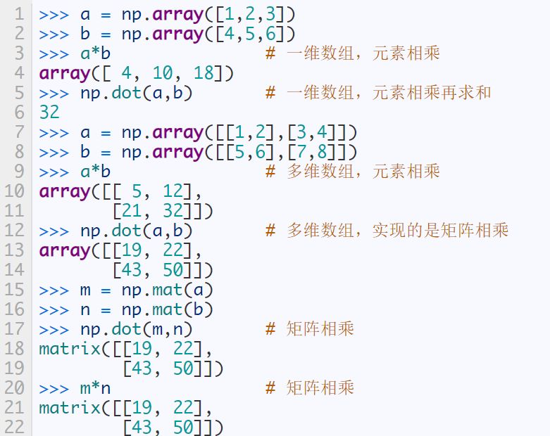
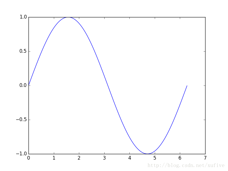
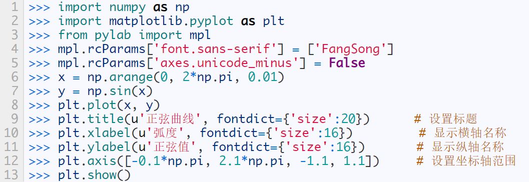
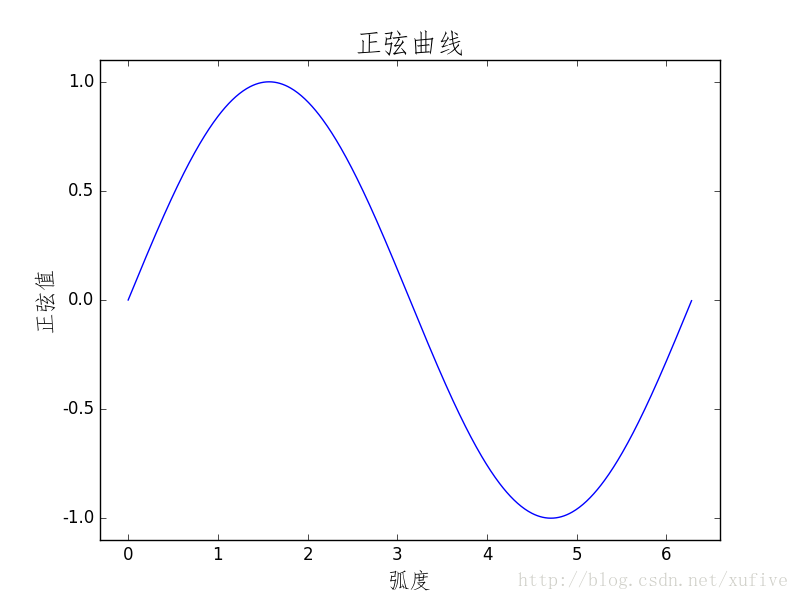
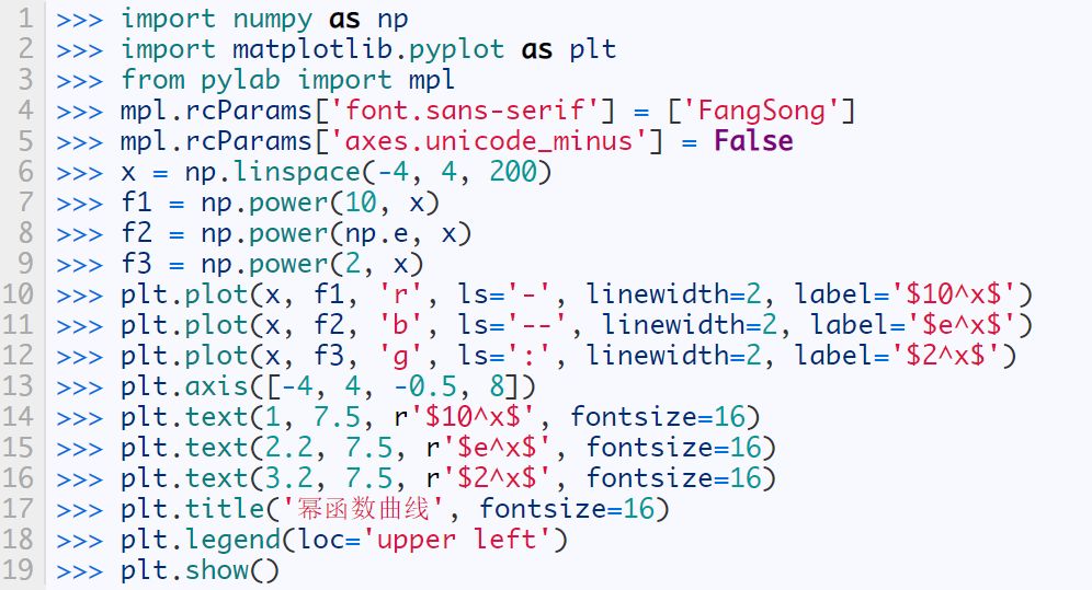
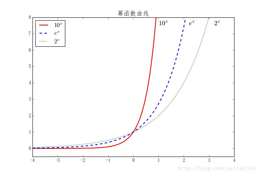
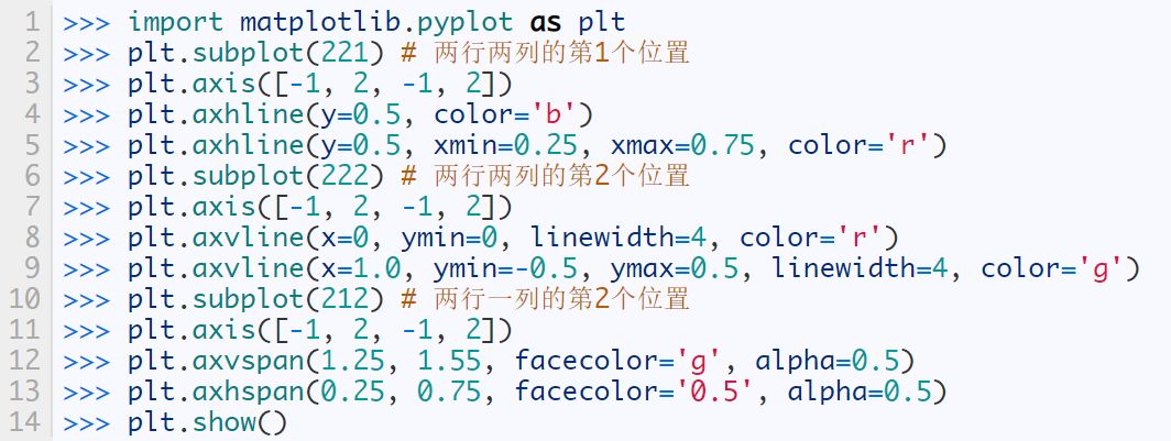
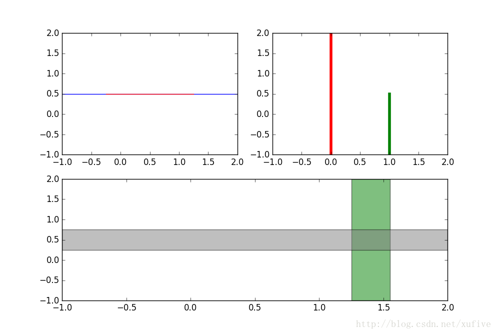
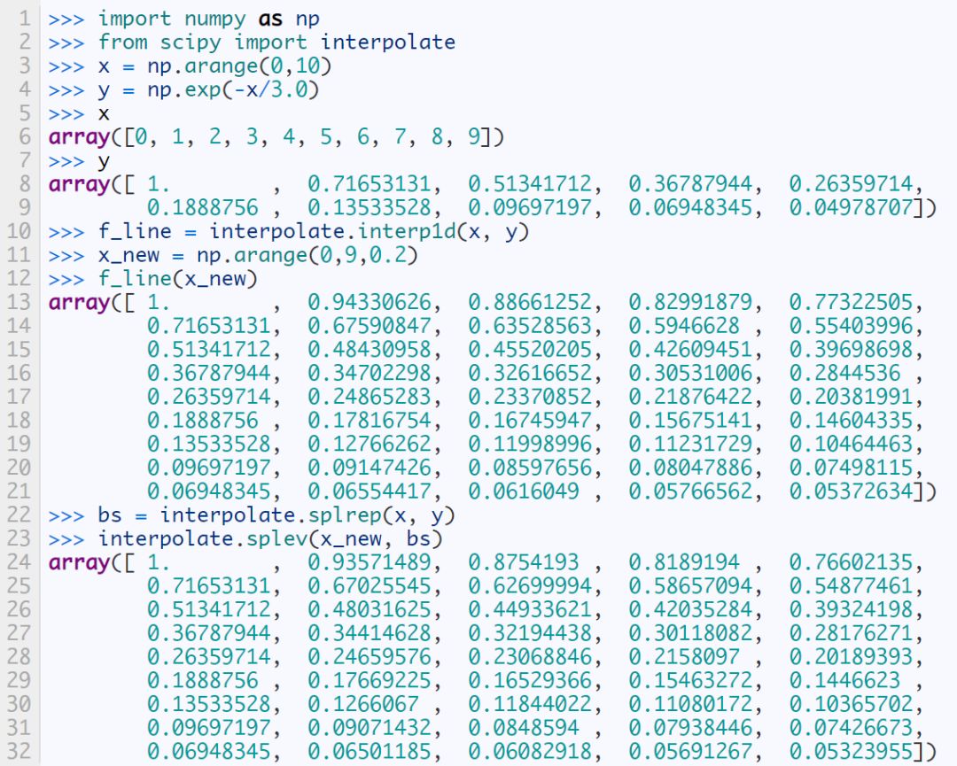
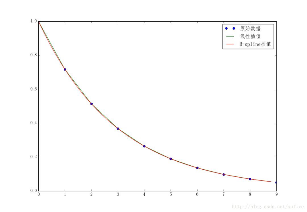
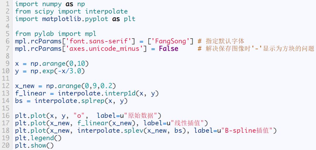
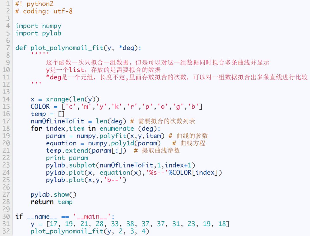
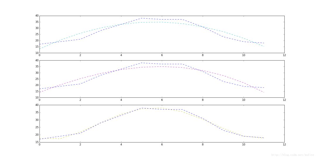
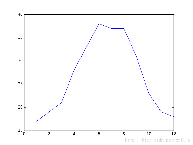
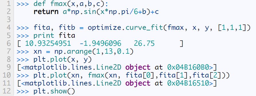
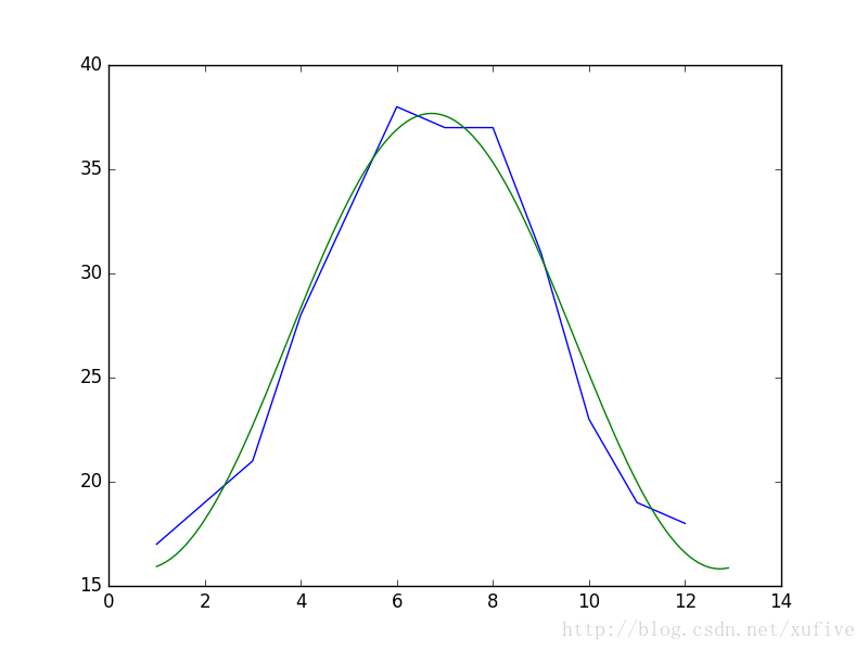
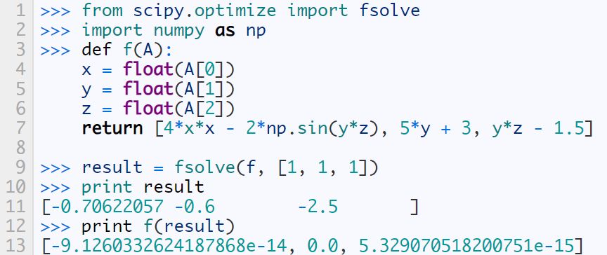
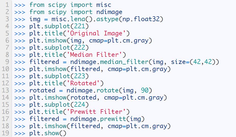
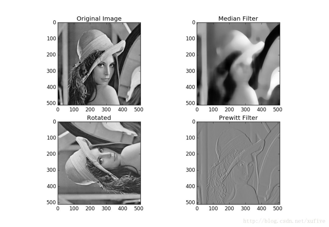
Whether you are a Barcelona fan or not, as long as you like football, you must have heard of the MSN combination of Messi, Suarez and Neymar. Among the many mathematical modeling aids, there is also an extremely sharp MSN combination. They are the famous Matplotlib + Scipy + Numpy three swordsmen under the command of python. This article is my MSN study notes. Some understanding may be superficial or even wrong. If this misleads a certain judge and causes major mistakes or losses at work, I can only compensate for one meal at most—and it must be our ten yuan box lunch downstairs. Hereby declare. The code in the article is copied from my Yoga 3 pro, which has troubles and angers from time to time. This means that all the codes can run smoothly in the following operating environment: pyhton 2.7.8 numpy 1.11.1 scipy 0.16.1 matplotlib 1.5.1 Numpy of the Three Musketeers numpy is an open source python scientific computing library, which contains many practical mathematical functions, covering functions such as linear algebra, Fourier transform and random number generation. The original numpy was actually part of scipy, and it was later separated from scipy. numpy is not a standard library of python and needs to be installed separately. Assuming that your operating environment has installed the python package management tool pip, the installation of numpy is very simple: pip install numpy Array object ndarray is a multidimensional array object and the core object of numpy. In numpy, the dimensions of an array are called axes, and the number of axes is called rank. Generally, all elements of a numpy array are the same type of data, and the storage of these data has nothing to do with the form of the array. The following example creates a three-dimensional array (when importing numpy, it is usually abbreviated as np). import numpy asnp a = np.array([[1,2,3],[4,5,6],[7,8,9]]) type of data The data types supported by numpy mainly include bool, integrate, float, and complex. Each data type is divided into several different types according to the number of bytes occupied by the memory. Subtype. The common data types are shown in the table below. Create an array Usually, we use np.array() to create an array. If you just create a one-dimensional array, you can also use the np.arange() or np.linspace() method. np.zeros(), np.ones(), np.eye() can construct special data. np.random.randint() and np.random.random() can construct an array of random numbers. Construct a complex array Many times, we need to construct complex arrays from simple data structures. For example, use one-dimensional data to generate two-dimensional grid points. Repeating array: tile One-dimensional array gridding: meshgrid Meshing with specified range and division method: mgrid Imaginary numbers are used in the above example. The method of constructing an imaginary number is as follows: >>> complex(2,5) (2+5j) Array attributes In addition to some regular attributes, numpy array objects also have several attributes that look more like methods, such as transpose and flat iterators. A flat iterator may be a concise way to traverse a multidimensional array. The following code gives an example. Change the array dimension The storage order of numpy arrays is irrelevant to the dimensions of the array, so changing the dimensions of the array is a very convenient operation. Except for resize(), this type of operation does not change the storage order of the array itself. Indexing and slicing For indexing and slicing one-dimensional arrays, numpy is the same as python's list, and even more flexible. Suppose there is a two-story building, and the rooms in each floor are 3 rows and 4 columns, then we can use a three-dimensional array to save the number of occupants in each room (of course, it can also be other numerical information such as room area). Array merge In addition to the horizontal merging, vertical merging, and deep merging described below, array merging also includes row merging, column merging, and concatenate(). If you are lazier than me, then only understand the first three methods, they are enough. Array split Splitting is the reverse process of merging. The concept is the same, but there is a slight difference: Array operations The four arithmetic operations of arrays and constants are the operations of each element of the array separately with constants; the four arithmetic operations of arrays and arrays are the operations of the corresponding elements of the two arrays (two arrays have the same shape, otherwise an exception will be thrown). Special note: If you want to do special treatment to the elements in the array that meet certain conditions, the following code may be useful. Array methods and commonly used functions The array object itself provides built-in methods such as calculating the arithmetic average and finding the maximum and minimum values, and numpy also provides many useful functions. In order to reduce the length, the following code only takes a one-dimensional array as an example to demonstrate the usage of these methods and functions. In fact, in most cases these methods and functions are equally effective for multidimensional arrays, with a few exceptions, such as the compress function. Matrix object Matrix is ​​a matrix object, inherited from the ndarray type, so it contains all the data attributes and methods of the ndarray. However, when you manipulate the matrix object as an array, you need to pay attention to the following points: The matrix object is always two-dimensional, even if it is a flattening (ravel function) operation or member selection, the return value is also two-dimensional The mixed operation of the matrix object and the ndarray object always returns the matrix object Create matrix The matrix object can be created using a Matlab-style string (a string separated by spaces and rows separated by semicolons), or it can be created using an array. Specific properties of the matrix The matrix has several unique properties that make calculations easier. These properties are: Matrix multiplication For the ndarray object, the asterisk is multiplied by the element, and the dot() function is treated as a matrix multiplication. For matrix objects, the asterisk and dot() functions are both matrix multiplication. In particular, for one-dimensional arrays, the dot() function implements a vector dot product (the result is a scalar), but the asterisk implements a difference multiplication. Linear Algebra Module numpy.linalg is the linear algebra module of numpy, which can be used to solve problems such as inverse matrix, eigenvalue, linear equation system and determinant. Calculate the inverse matrix Although the matrix object itself has the attribute of the inverse matrix, it is very simple to use the numpy.linalg module to solve the inverse of the matrix. Calculate the determinant I don't remember how to calculate the determinant, but I still remember the pain of manually calculating the determinant. Now it's good, you can easily do it with numpy on your phone (provided that python + numpy is installed on your phone). m = np.mat('0 1 2; 1 0 3; 4 -3 8') np.linalg.det(m)# What? Is this done? 2.0 Calculate eigenvalues ​​and eigenvectors So far, my work has nothing to do with eigenvalues ​​and eigenvectors. Recording this section is purely for my daughter, who is studying mathematics. Solve a system of linear equations There are linear equations as follows: x – 2y + z = 02y -8z = 8-4x + 5y + 9z = -9 The solution process is as follows: Matplotlib of the Three Musketeers matplotlib is the most famous plotting library in python. It provides a set of command APIs similar to Matlab, which is very suitable for interactive drawing. And it can be easily used as a drawing control and embedded in GUI applications. matplotlib can draw various forms of graphs, including ordinary line graphs, histograms, pie graphs, scatter graphs, error bar graphs, etc.; various properties of the graph can be easily customized, such as line type, color, thickness, font It can well support some TeX typesetting commands, and can display mathematical formulas in graphics more beautifully. Introduction to pyplot Matplotlib contains dozens of different modules, such as matlab, mathtext, finance, dates, etc., and pyplot is our most commonly used drawing module, which is also the focus of this article. Solution to Chinese display problem There are many ways to solve this problem, but the following method is probably the simplest solution (I only tested it on the windows platform, please see the official self-test for other platforms). Draw the simplest graph >>> import numpy asnp >>> import matplotlib.pyplot asplt >>> x = np.arange(0,2*np.pi,0.01) >>> y = np.sin(x) >>> plt.plot(x,y) >>> plt.show() Set title, axis name, axis range If you run the following code in a python shell, and the default encoding of the shell is not utf-8, the Chinese may still be displayed as garbled characters. You can try to write u'sine curve as'sine curve'.decode('gbk') or'sine curve'.decode('utf-8') Set the style, width and color of points and lines The calling form of plt.plot function is as follows: plot(x,y,color='green',linestyle='dashed',linewidth=1,marker='o',markerfacecolor='blue',markersize=6) plot(x,y,c='g',ls='--',lw=1,marker='o',mfc='blue',ms=6) color specifies the color of the line, which can be abbreviated as "c". The color options are: Blue:'b' (blue) Green:'g' (green) Red:'r' (red) Dark green:'c' (cyan) Magenta:'m' (magenta) Yellow:'y' (yellow) Black:'k' (black) White:'w' (white) Grayscale representation: eg 0.75 (any floating point number within [0,1]) RGB notation: eg'#2F4F4F' or (0.18, 0.31, 0.31) linestyle specifies the line style, which can be abbreviated as "ls". The line type options are: Solid line:'-' (solid line) Dotted line:'–' (dashed line) Dash-dot line:'-.' (dash-dot line) Dotted line:':' (dotted line) None: "or" or "None" linewidth specifies the line width, which can be abbreviated as "lw". The marker describes the shape of the data point Dotted line: '.' Dotted line:'o' Plus sign:'+ Cross:'x' Upper triangle:'^' Upper triangle:'v' markerfacecolor specifies the surface color of the data point marker, which can be abbreviated as "mfc". markersize specifies the size of the data point marker, which can be abbreviated as "ms". Text annotations and legends We use different line types and colors to draw a set of power function curves based on 10, e, and 2 to demonstrate the use of text annotations and legends. When drawing the legend, loc is used to specify the position of the legend, the available options are: best upper right upper left lower left lower right Draw a multi-axis graph While introducing how to draw multiple sub-pictures on the same drawing board, by the way, demonstrate how to draw straight lines and rectangles. We can use the subplot function to quickly draw a chart with multiple axes. The calling form of the subplot function is as follows: subplot(numRows, numCols, plotNum) The subplot divides the entire drawing area into numRows rows * numCols column sub-areas, and then numbers each sub-areas in the order from left to right and top to bottom, and the number of the upper left sub-areas is 1. If numRows, numCols and plotNum are all less than 10, they can be abbreviated as an integer. For example, subplot(323) and subplot(3,2,3) are the same. subplot creates an axis object in the area specified by plotNum. If the newly created axis overlaps with the previously created axis, the previous axis will be deleted. Scipy of the Three Musketeers As mentioned earlier, the original numpy was actually part of scipy, which was later separated from scipy. The scipy function library adds many library functions commonly used in mathematics, science and engineering calculations on the basis of the numpy library. For example, linear algebra, numerical solution of ordinary differential equations, signal processing, image processing, sparse matrix and so on. Because of the many fields involved, I am like scipy to scipy, like a blind person touching an elephant, I can only count wherever I touch it. Interpolation One-dimensional interpolation and two-dimensional interpolation are one of the most commonly used functions of scipy, and they are also the easiest to use. One-dimensional interpolation and spline interpolation The following example clearly shows the data shape after linear interpolation and spline interpolation. Plot the original data and the data after linear interpolation and spline interpolation together, the effect will be more obvious: code show as below: Special note: Spline interpolation comes with many default parameters. The following is a brief description. Please search for details yourself. scipy.interpolate.splrep(x,y,w=None,xb=None,xe=None,k=3,task=0,s=None,t=None,full_output=0,per=0,quiet=1) # The parameter s is used to determine the number of smoothing points, usually m-SQRT(2m), where m is the number of curve points. If smoothing is not needed in interpolation, s=0 should be set. The output of splrep() is a 3-element cell array (t, c, k), where t is the curve point, c is the calculated coefficient, and k is the order of the spline, usually 3, but it can be passed through k change. scipy.interpolate.splev(x,tck,der=0) # The der is the order that needs to be actually calculated for the spline calculation, and the condition der must be met Fit In work, we often need to use a curve to fit these actual data while depicting some actual data observations in the graph. The so-called fitting is to find out the curve equation that conforms to the trend of the data, or directly draw the fitting curve. Fitting using numpy.polyfit The following code, based on the Numpy module, can directly draw the fitted curve, but I cannot get the curve equation (although it outputs a bunch of curve parameters). This is a question worthy of further study. The 3 fitting results are shown in the figure below. Use scipy.optimize.optimize.curve_fit to fit The fitting provided by scipy seems to need to determine the curve equation with parameters first, and then scipy solves the equation and returns the curve parameters. We still use the above set of data as an example to use scipy to fit the curve. It can be seen that the curve approximates a sine function. Construct the function y=a*sin(x*pi/6+b)+c, and use the optimize.curve_fit function of scipy to find the values ​​of a, b, and c: Solve nonlinear equations (sets) In mathematical modeling, some weird equations (sets) need to be solved. Matlab is naturally the first choice, but Matlab is not free, and scipy provides us with free lunch! The fsolve function in the scipy.optimize library can be used to solve nonlinear equations (sets). Its basic calling form is as follows: fsolve(func, x0) func(x) is a function for calculating the error of the equation system. Its parameter x is a vector, which represents a set of possible solutions for each unknown number of the equation system. Func returns the error obtained after substituting x into the equation system; x0 is the initial value of the unknown number vector value. Let’s solve a simple equation first: sin(x)−cos(x)=0.2 >>> from scipy.optimize import fsolve >>> import numpy asnp >>> deff(A): x = float(A[0]) return[np.sin(x)-np.cos(x)-0.2] >>> result = fsolve(f,[1]) array([0.92729522]) >>> print result [0.92729522] >>> printf(result) [2.7977428707082197e-09] Haha, it's easy! Here is another set of equations: 4x2−2sin(yz)=0 5y+3=0 yz−1.5=0 Image Processing In the scipy.misc module, there is a function to load a Lena image-this image is a classic demonstration image used for image processing. I just briefly show a few operations on the image. Load Lena image and display grayscale image Apply median filter to scan each data point of the signal and replace it with the median value of adjacent data points Rotate image Apply Prewitt filter (gradient calculation based on image intensity) postscript This blog post has been written intermittently for more than 5 months since the beginning of September 2016. The delay for so long was mainly due to the fact that the subject of MSN was too complicated and extremely obscure, in addition to its own laziness. No matter how hard you tried, I was always afraid to make a mistake and laugh at it generously. The advantage of USB Cable Type C is that it supports higher current, that is that more current can be passed by Type-C in the same time. In this way, the charging speed of the device can be accelerated. At present, the charging current of most Type-C data lines is generally 2A. If the charging rate of 3A is to be reached, a high-current wall charging matching it is required. That is to say, if the wall charge only supports 1A, whether it is charged with 2A or 3A data line, there is no difference fundamentally. If the current supported by the wall charging is 2A, and the type-C data cable of 2A/3A is matched, the effect can be significantly changed.
The highlights of Type-C interface are thinner design, faster transmission speed (USB3.1 up to 10Gbps) and stronger power transmission (up to 100W).The biggest feature of Type-C double-sided plugable interface is that it supports double-sided insertion of USBinterface. Officially solved the USB never insert the worldwide problem, the front and the back of the random plug.The USB Cable used with it must also be thinner and lighter.
Usb Cable Type C,Usb Type C Cable,Type C 3.0 Cable,Usb Type C Data Cable Henan Yijiao Trading Co., Ltd , https://www.yjusbhubs.com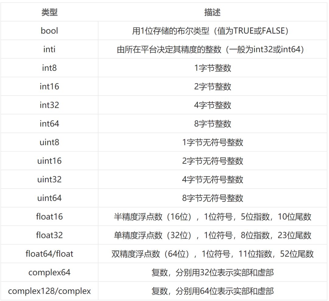












In addition, the device equipped with the Type-C interface can be charged by connecting the mobile power supply through the Type-C cable or Usb C Cable. Users do not need to carry the charging cable, but can have the wall charging and Type-C cable. In addition, when selecting a Type-C charging cable, We should pay attention to the current limit. The charging data cable 1A does not have fast charging performance, 2A is the most commonly used Type-C charging data line, and 3A is the best data line at present. If you want to have fast charging effect, you must choose the Type-C charging data line with 3A current.
